COMPSCI 184 Project3: PathTracer

Part 0: Project overview

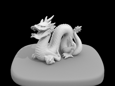
In this project, I implemented some fundamental functions and features of a physically-based renderer using path tracing algorithm. First, I implemented ray generation and the intersection between ray and objects/scene. Next, I implemented the BVH splitting and intersection detection. Then, I implemented direct illumination(zero/one bounce lights) and global illumination(multi-bounce lights w/ w/o russian roullete) to actually render the whole scene with path tracing. Finally, I implemented adaptive sampling to reduce the noise of monte carlo path tracing.

Part 1: Ray Generation and Scene Intersection

Ray generation walkthrough & primitive intersection pipeline

I first calculate the bottom left and the top right corner of the sensor/image space coordinates, which helps me to determine the coordinates in the camera space with left multiplcation of the c2w matrix. Then with the origin pos and the previously calculated coord as direction vector(since the origin is [0,0,0] and it’s numerically the same for the coords and the vector), we can generate the correct ray.

Primitive is the bridge between geometry processing and the shading subsystem. It contains all the things including bbox, intersect, has_intersection and bsdf. For intersections, we use has_intersection to determine whether it’s intersected or not and use intersect to actually change the intersection distance, the normal vector, and the bsdf.

Triangle intersection algorithm walkthrough

For the intersect and has_intersection, I used the Moller-Trumbore algorithm to compute them. We compute two edges of the triangle. Compute the determinant det to check if the ray is nearly parallel. Compute u and v(barycentric coordinates) to ensure the intersection lies within the triangle. Compute t, the intersection distance along the ray. And finally check if t is within the ray’s valid range (min_t to max_t). The function intersect basically determine whether has_intersection is true or not and change the primitives and the properties mentioned above(intersection distance, normal vector, bsdf).

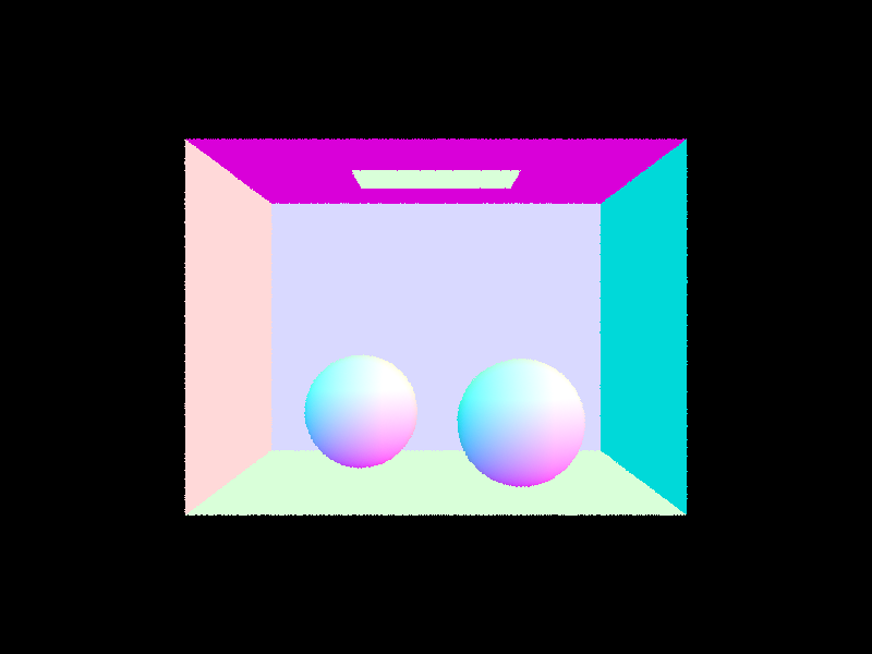
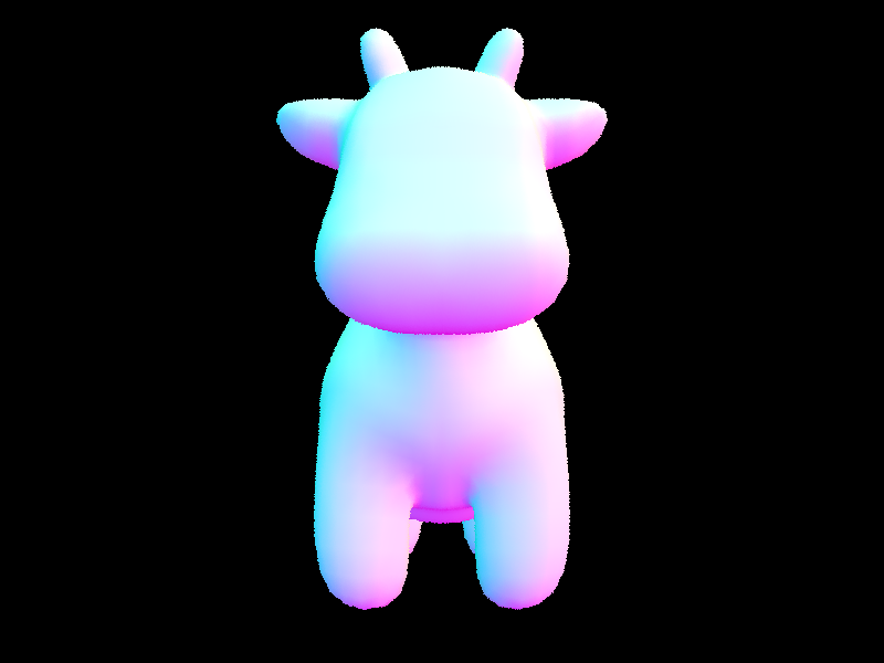
Some results

CB spheres	cow

Part 2: Bounding Volume Hierarchy

BVH construction algorithm walkthrough

First, compute the bounding box (BBox) of all primitives in the given range [start, end). Then, I choose the best axis to split: compute the bounding box centroid for each primitive. Select the axis with the largest extent (X, Y, or Z) and split at the centroid median to achieve balanced partitions. The primitives are sorted first and partitioned into left and right subsets. Finally, recursively call function and construct BVH for left and right subsets and return the newly created BVHNode.

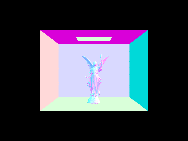
Some results

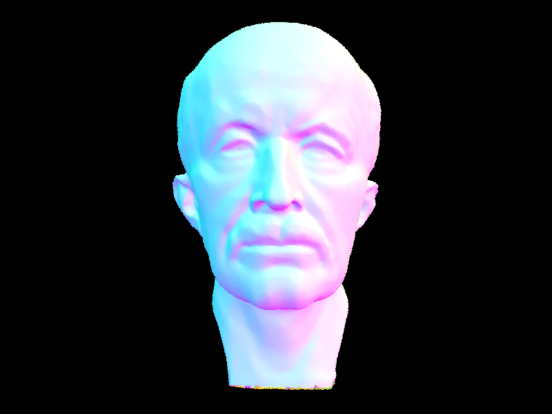
CB Lucy	Max Planck

More on BVH acceleration

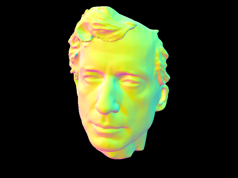
First, here’s more result on the BVH rendering(left) and the comparison between the non-BVH. You can see that there’s basically no difference between them.

Peter w/ BVH	Peter w/o BVH

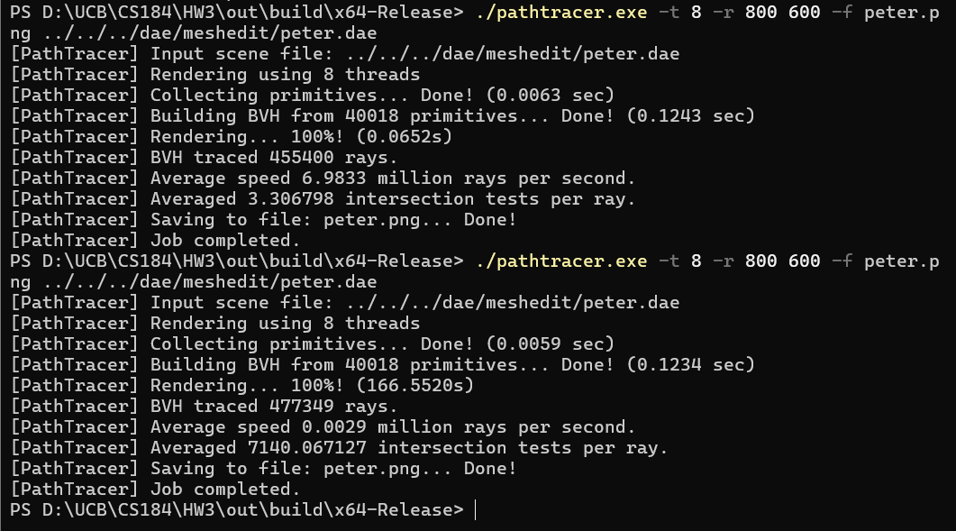
But the rendering time, as shown in the picture below, have significant difference. One is 0.0653 second, and the other takes 166.5520 seconds to finish. Nearly 300x faster.

Part 3: Direct Illumination

Direct Lighting functions walkthrough

Uniform Hemisphere Sampling

In the loop of num_sample samples, we sample from hemisphereSampler, then we create a new ray with in point hit_p and the epsilon constant for avoiding numerical presision issues and direction sampled earlier. If the ray intersects we calculate the L_out of the ray. Finally we divide the sum of all the things above with pdf and the num_samples.

Importance Sampling Lights

FOr importance sampling, we sample all the lights directly After we calculate the hit point hit_p, we directly sample a light ray from it. If we cast a ray in this direction and there is no other object between the hit point and the light source, then we know that this light source does cast light onto the hit point. After the judge, we still do the same thing as above(divide the sum of all the things above with pdf and the num_samples).

Some results

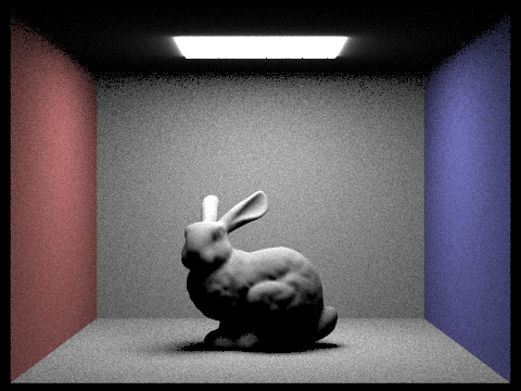
Hemisphere uniform sampling	Direct importance sampling

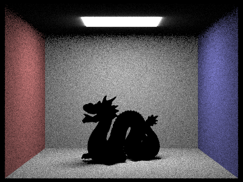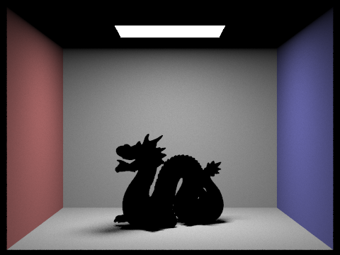Hemisphere uniform sampling	Direct importance sampling

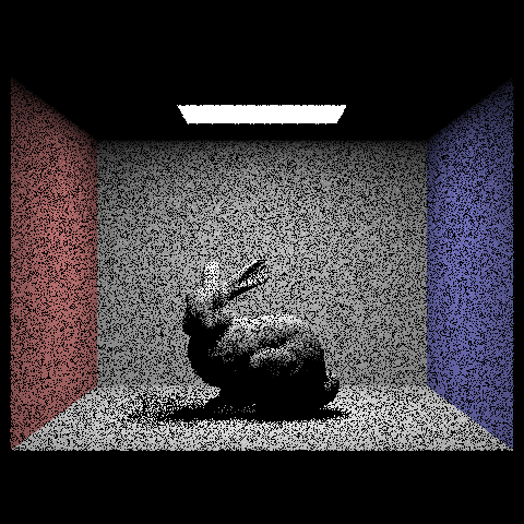
Direct comparison

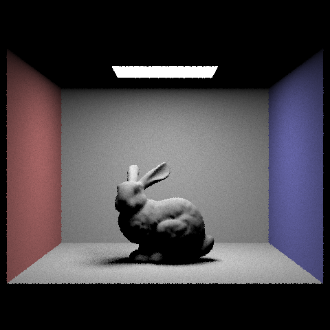Up 1 Down 16	Up 4 Down 64

Conclusion

Uniform hemisphere sampling distributes samples evenly over the hemisphere, leading to significant variance in Monte Carlo integration when evaluating lighting contributions, especially in scenes with strong directional lighting. This results in more noise and slower convergence. In contrast, importance sampling strategically places more samples in directions where the light source contributes most to the radiance, reducing variance and improving efficiency. This method converges faster, producing smoother and more accurate results with fewer samples.

Part 4: Global Illumination

Indirect lighting function walkthough

We get the one bounce radiance first, then, we sample a new f using the outgoing direction of the last ray. We create new ray and increase its depth by 1. When the depth reaches the max depth, just return the one bounce result earlier(this is the last one being calculated), otherwise recursively calling the function.

As for russian roulette, the difference is that every new ray generated each turn has to pass the russian roulette coin flip check in order to not be eliminated and thrown away. The probability I’m using here is 70% continue, 30% delete each turn.

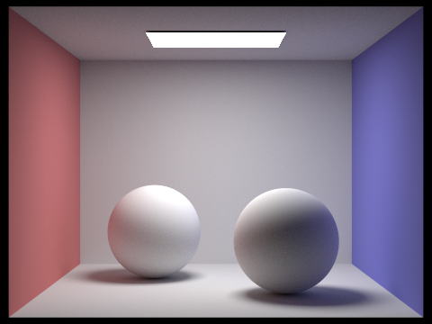
Some global illumination results

Bunny (maxdepth=2)	Spheres (maxdepth=4)

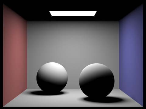
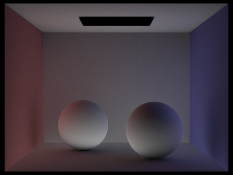
Only direct illumination vs. only indirect illumination

only direct illumination	only indirect illumination (maxdepth=2)

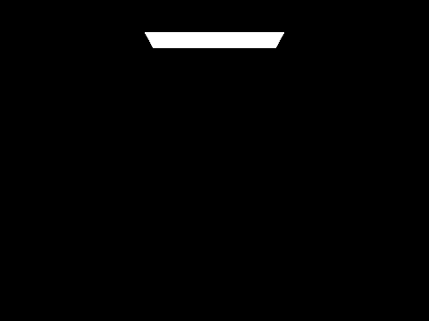
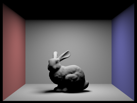
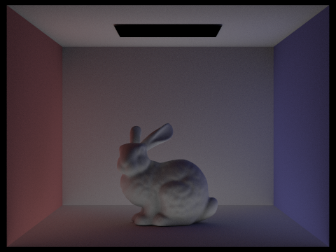
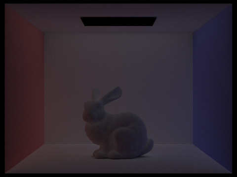
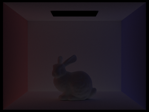
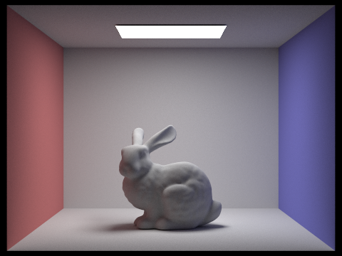
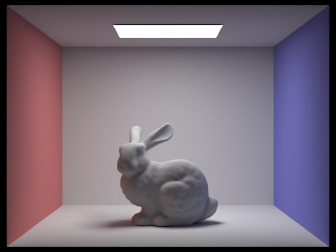
Renders of max_ray_depth from 0 to 5

specs using: -t 12 -s 1024 -l 8 -r 480 360, click the image to zoom in on the website.

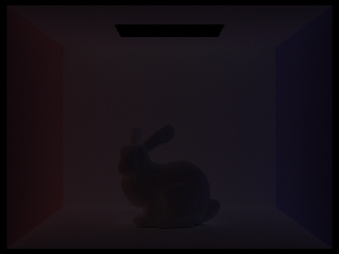
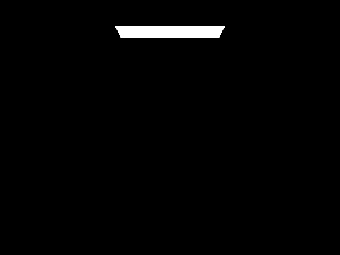
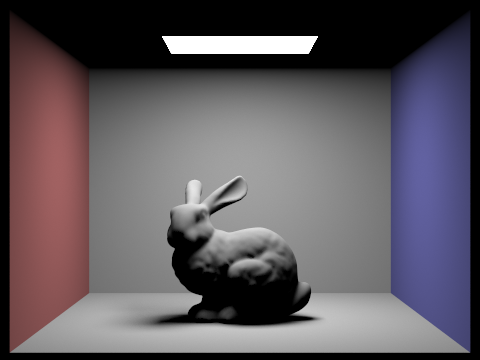
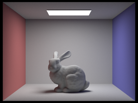
isAccumBounces	m = 0	m = 1	m = 2	m = 3	m = 4	m = 5
false
true

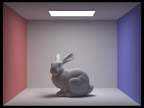the 2nd and 3rd bounce of light

For the 2nd bounce of the light, its main contribution is that it illuminates the ceiling, making the overall rasterization way more realistic. For the third bounce of light, it slightly illuminates the ground around the bunny, mimicing the lights reflected away from the bunny surface, making the overall rasterization more realistic.

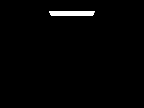
Russian roulette rendering results

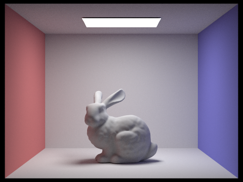
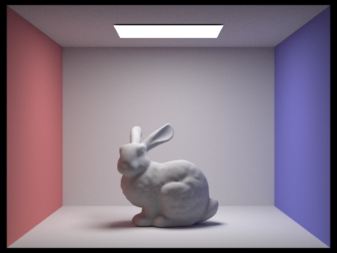
specs using: -s 1024 -l 4. Along with using russian soulette, you may not be able to see that much difference after 2 bounce.

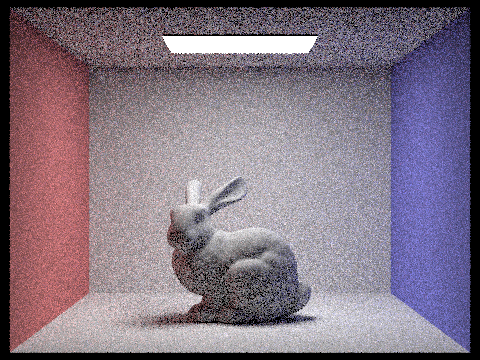
Various sample-per-pixel rates results

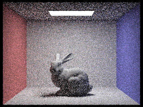
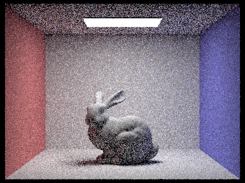
From left to right, from top to bottom: 1 2 4 8 16 64 1024.

Part 5: Adaptive Sampling

Adaptive sampling walkthrough

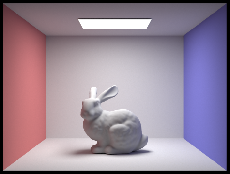
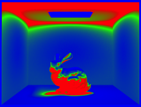
Adaptive sampling is a method used in ray tracing to reduce the number of samples per pixel while maintaining image quality. Instead of taking a fixed number of samples (ns_aa), it dynamically decides when to stop sampling based on statistical analysis.

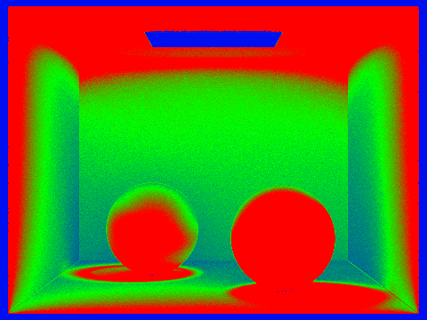
(If only one sample is requested, the algorithm traces a single ray and directly stores the computed radiance.) We loop over ns_aa samples, and only check after every samplesPerBatch samples. Then we calculate and check confidence interval I is smaller or larger than a threshold, if smaller then it stops early. otherwise just like ordinary calculation. Once sampling is complete (either because the pixel converged or the maximum samples were taken), the final radiance is computed as the average of all collected samples.

Some results

bunny	bunnyrate

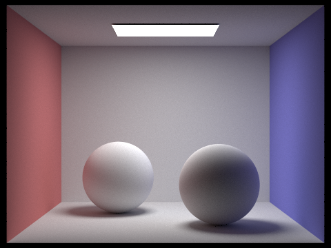
ball	ballrate